Papers & Code

Rules in the GSOS format are natural transformations, and their models are bialgebras. For a simple distributive law $\lambda :\mathrm{\Sigma }B\Rightarrow B\mathrm{\Sigma }$, the comonad $G=FU$ of free bialgebras resolves every model, and a coefficient functor turns the resolution into a chain complex. Its homology $H_n^{\lambda }(X;M)$ is the comonad homology of Barr and Beck. For linear rules with observational coefficients it reduces to two groups, and one Smith normal form computes them. In degree one it finds laws that hold in a model but not in the free one, such as $\rho (\rho (x))=x$.

Finite clopen partitions of the nerve cut finite chain models out of the Matui complex. Helly conditions on the covers constrain nothing. Laminar presentations bound the rank of a model by the size of the cover and give a complete system of models for every second countable Hausdorff ample groupoid. No finite model is a resolution in general, since $H_0$ over $\mathbb{Z}$ is not finitely generated for the Cantor set.

A quantitative equational theory $U$ gives every metric space $A$ a free algebra $T_{U}A$, measured by the least distances the axioms derive. Filtering its length nerve by length yields a persistence module whose associated graded is the magnitude complex, and a long exact sequence joins the two. Magnitude homology then tells where bars can begin and end. The barcode in degree $n$ moves by at most $(n+1)\delta$ under a perturbation of size $\delta$, and an example shows that the factor $n+1$ is needed. When added axioms keep the free algebra the same set, the barcode moves by at most $n+1$ times the change of metric.

A task is a small category, a change of task is a functor $J:\mathcal{A}\to \mathcal{B}$, and a representation is a functor $F:\mathcal{A}\to \mathcal{V}$ into invariants. The left Kan extension ${\mathrm{Lan}}_{J}F$ is the structure the new task has to carry, so a target $G$ is scored by its largest distance to ${\mathrm{Lan}}_{J}F$ over the objects of $\mathcal{B}$. The extension has cokernel presentations in chain complexes and in persistence modules. For one-parameter modules of finite type the score is exactly the bottleneck distance.

The map $C_{\bullet }(\mathcal{G};\mathbb{Z}){\otimes }_{\mathbb{Z}}A\to C_{\bullet }(\mathcal{G};A)$ is always injective, and it is surjective if and only if every compactly supported continuous map into $A$ is locally constant. The universal coefficient theorem for ample groupoids is therefore about discrete coefficients, and it fails for $\mathbb{R}$ on the Cantor set. Clopen invariant covers make the Mayer–Vietoris sequence trivial. Open invariant covers give a working sequence for every coefficient group, with a nonzero connecting map already for an integer action on the two-point compactification of $\mathbb{Z}$.

Matui-type homology is built from compactly supported, locally constant chains on the nerve. For a discrete group it is the homology of the classifying space, but for a space seen as a groupoid of units it computes compactly supported cohomology. On the Cantor set $X$ the two differ already in degree zero: $H_0(\mathcal{G};\mathbb{Z})\cong C(X,\mathbb{Z})$ is countable, while $H_0^{\mathrm{sing}}(B\mathcal{G};\mathbb{Z})$ has cardinality $2^{{\mathrm{\aleph }}_0}$. In every positive degree they agree.

Homology of ample groupoids with coefficients in a topological abelian group $A$, functorial and invariant under Kakutani equivalence. For discrete $A$ the universal coefficient sequence follows from the isomorphism $C_c({\mathcal{G}}_n,\mathbb{Z}){\otimes }_{\mathbb{Z}}A\cong C_c({\mathcal{G}}_n,A)$. In general, the image of this map consists of the compactly supported maps with finite image.

From simplicial and singular homology, exact sequences and excision to persistent homology and persistent cohomology of filtrations, with many proofs written anew.

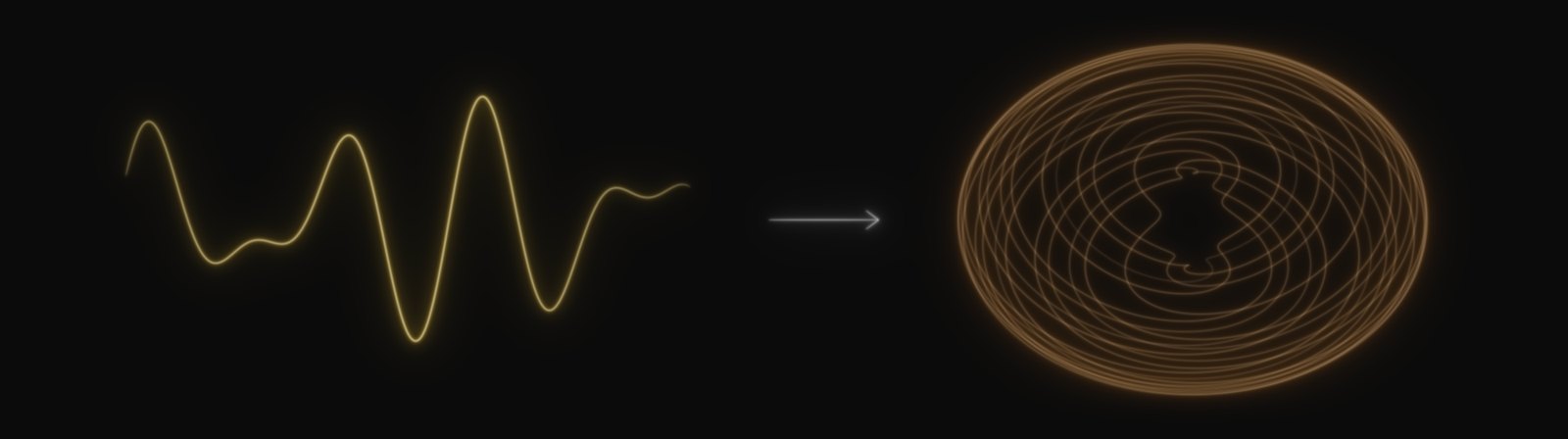
Sliding windows turn sensor signals into point clouds, and their Vietoris–Rips persistence gives Betti curves in degrees $0$ and $1$. A network with three branches reads the raw signal and both curves and assigns each signal its designation in the plant.

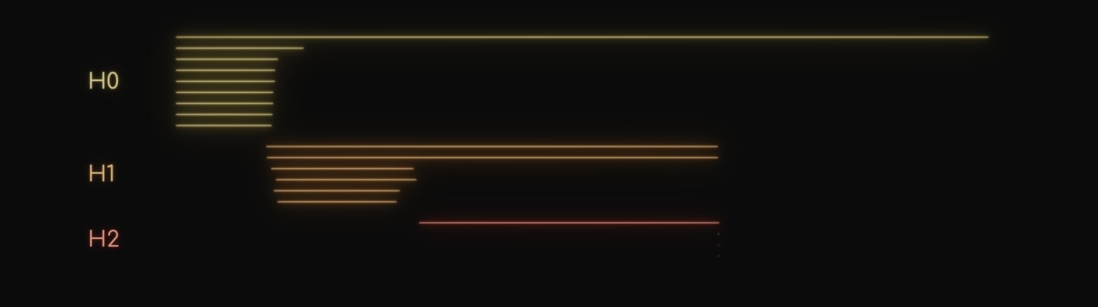
If the data live on a connected abelian Lie group, that group is ${\mathbb{T}}^q\times {\mathbb{R}}^p$, and its Betti numbers $(\genfrac{}{}{0ex}{}{q}{k})$ determine $q$. Reading them off persistence landscapes gives a lower bound for the width of a network layer.

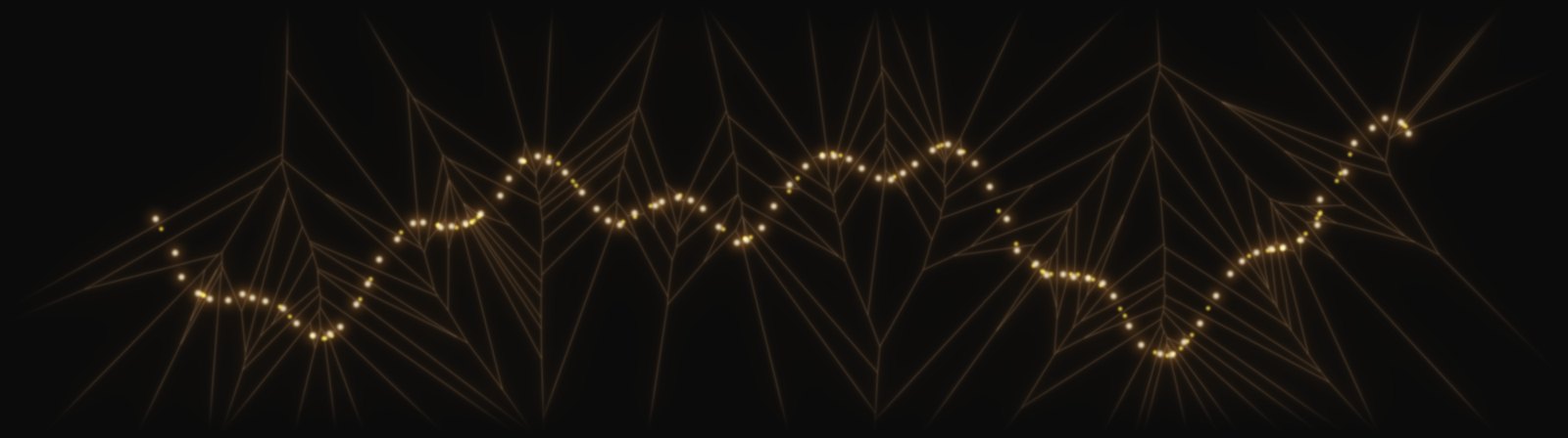
Natural-neighbour interpolation keeps adding points, and sooner or later it changes the topology of the data. Comparing the persistence diagrams of consecutive steps tells it when to stop.

In radionuclide therapy with ${}^{177}\mathrm{Lu}$, a single dose kernel ignores differences between tissues, and Monte Carlo transport is slow. A U-residual network learns the map from local density to dose kernel instead. On unseen patients it reaches a continuous intersection over union of 0.86.

A sociolinguistic case study, in German, of brauchen with and without zu before an infinitive.